How to Read Pump Curve? Performace, Characteristic Curve for Centrifugal Pump

What is Pump curve? Or How to read pump curve? MechStudies helps you understand how pump curves can provide relevant information about the pump’s efficiency and brake horsepower.

Let’s explore the Pump Characteristics Curve!

What is Pump Characteristic Curve?

Let’s start the pump curve or pump characteristic curve with basics, definitions, and examples.

Definition of Pump Curve

The pump characteristic curve is defined as ‘the graphical representation of a particular pump’s behavior and performance under different operating conditions.

Pumps come in different sizes based on their power and flow rate. Reading and understanding centrifugal pump curves is important in selecting the most reliable and efficient pump in various industries.

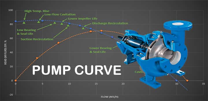
Don’s worry about the above image, we will learn all the basics of pump curve.

Why Do We Need to Study Pump Characteristic Curve?

Let’s try to understand why do we need to study the pump curve? The reasons are as follows,

• Selecting the correct pump maximizes your hydraulic system performance and it’s very crucial for the application it will be used in.
• Selecting the wrong pump will lead to increased inefficiency and eventually premature failure in pump operations.
• If the pump is running out of curve it denotes that there’s cavitation inside the pump and wear of the impeller and bearings will happen.
• Curve interpretations help in making decisions about – choice of pump, motor sizing, and power consumption strategies.

Terminologies of Pump Curve

Before starting, let us understand some basic terms associated with pump curves:

• Impeller: It’s a rotating component of a centrifugal pump that pushes the fluid outwards.
• Volute: It’s a pump casing that collects the fluid discharged by an impeller.
• Head: It’s a measure of pressure or force exerted by water expressed in feet.
• Static Head: The vertical height difference between the surface of the water and the center of an impeller is a static head.
• Total Head: Total head is measured by measuring the distance from the source of water surface to the output of the pump.
• Flow Rate: The amount of liquid that can be carried in a given time, usually measured in gpm, cpm, etc.
• Net Positive Suction Head: The amount of suction lift that can be generated by creating a vacuum.
• Cavitation: Cavities or voids in the pump casing. Bubbles forming inside the pump casing take up space and decrease the pump capacity. These bubbles damage the impeller and volute casing making cavitation a problem for pump and seal both.

Pump Curve Basics

Before going to understand the pump curve as well as pump characteristic curve, let’s explore,

Pump Curve Axis

As pump is a graphical representation, the x-axis is used to denote pump head and y-axis is used to denote pump flow rate.

The pump head in layman’s language is nothing but the pressure produced by the pump and flow rate means the quantity of liquid flow per hour.

• The pump head is denoted by H
• Pump flow rate is denoted by Q
• Unit of the pump head is meter (m), or feet (ft),
• Unit of flow rate is m3/hr or liter/s (lps) or gallons per minute (GPM)

Formation of Pump Curve

Let’s see how a pump curve is formed to understand practically. We will consider Q =20 m³/hr for the pump and try to find out the behavior of the pump.

• Case-1

If Q amount of water is supplied to a pump for transferring this water horizontally, then its head will be zero and the discharge will be Q1.

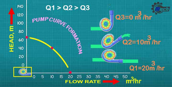
Hence, supply water flow rate (Q) = discharge water flow rate (Q1)

• Case-2

Now, if we rotate the centrifugal pump at 45 deg. angle anticlockwise then do you think Q amount of water will be transferred at discharge?

No, not possible, the amount of water will be reduced. Here, it is Q2=10 m³/hr

Hence, supply water flow rate (Q) > discharge water flow rate (Q2)

• Case-3

Now, again if we rotate the centrifugal pump at 90 deg. angle anticlockwise, what do you think about the discharge, Q3?

It will be zero, which means no water will be transferred. So, Q3=0.

Hence, supply water flow rate (Q=20m³/hr) > discharge water flow rate (Q2=10m³/hr) >discharge water flow rate (Q3=0)

Impeller Size in Pump Curve

The flow rate, as well as performance of the pump, depends on the impeller size of the centrifugal pump.

• If impeller size is more, it can increase more pressure.
• Size of impeller depends on the manufacturers as well as project requirements.

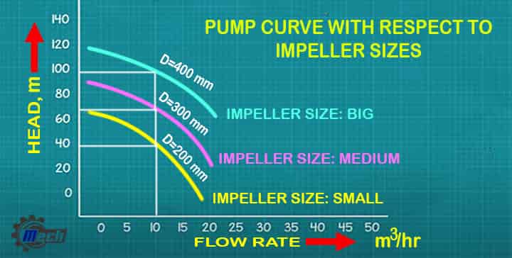
For example, we will take three different impellers for the pump and plot head with respect to capacity.

Impeller sizes are,

• 400 mm
• 300 mm
• 200 mm

Flow rate 10 m³/hr corresponding to below,

• Impeller 400 mm size, Head = 95 m
• Impeller 300 mm size, Head = 66 m
• Impeller 200 mm size, Head = 37 m

Now, selection shall be based on the project requirements. In case, the requirement of the head lies between two impeller sizes, machining to be done by the manufacturers.

Power in Pump Curve

Power requirement is one of the vital parts of the pump curve. It is for the selection of pump motor.

• If flow rate is increased, pump has to work more, means power requirement will be more.
• If flow rate is less, power requirement will be less.

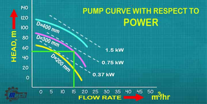
For example, three different pump curves, and flow rate is 15 m3/hr and the corresponding head is 52 m.

Now, this point lies between two power, 0.37 kW and 1.5 kW. Now, if we select 0.37 kW, pump will not work properly as its requirement is more than 0.37 kW but less than 1.5 kW.

In this case, we have to select the higher one considering the highest performance requirements as well as margin.

Efficiency in Pump Curve

Now, depending on impeller sizes, pump construction, head, flow, etc. pump efficiency is varied.

• Efficiency is plotted in the pump curve.
• Different impeller gives different efficiency.

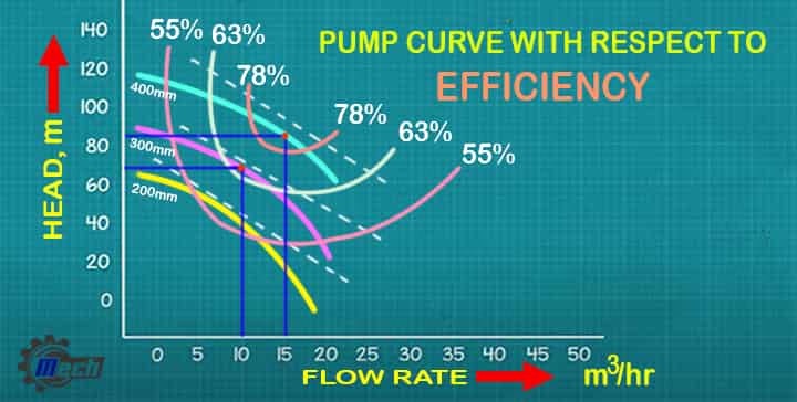
Refer to the image, here, the pump of 300 mm impeller size with a flow rate of 10 m³/hr and head 68 m, gives efficiency 64%

However, when the same pump select with a flow rate of 15 m³/hr and head 83 m, gives a higher efficiency 80%.

Hence, pump selection should be done considering the efficiency.

Special Note:

The pump efficiency curve looks different for a particular impeller size, as it derived by the manufacturer to get the flow rate with respect to efficiency for a particular impeller.

Few of them are illustrated based on the highest rating as well as feedback:

Centrifugal pumps: Principles, Operation and Design

Centrifugal Pump Basics (Mechanical Engineering & HVAC)

Introduction to Centrifugal Pumps (HVAC and Engineering)

Pump Characteristic Curve Example

Let’s see a look of a typical pump curve, indicating,

• Pump curve
• Operating point
• System curve
• Flow rate
• Static head, etc.

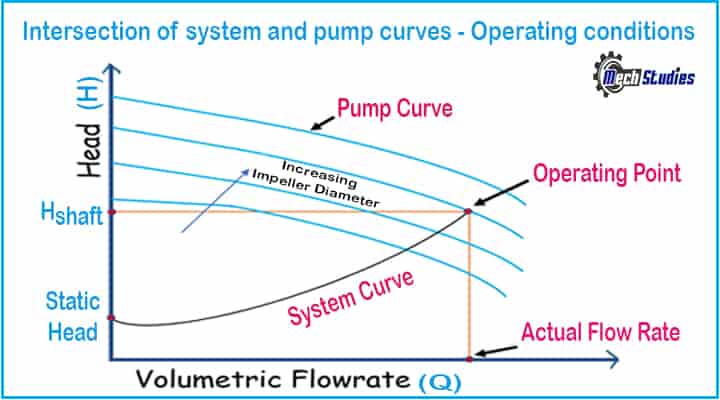
Refer few important special notes,

• The Intersection of system and pump curves determines its operating conditions
• The Pump curve is provided by the manufacturers
• System curve is based on the mechanical energy balance

Pump Characteristic Curve Classification

Pump curves are classified into three types,

• Q/H curve
• Efficiency curve
• NPSH curve

The pump is designed to run at the same speed as its prime mover which is usually an AC electric induction motor.

• In case of power failure or motor failure, the standby pump is coupled with a diesel engine for continuous operation.
• Running pumps using an engine allows variable speeds, in such situations, it’s important to know the performance of pumps at different speeds.

This can be determined by studying the characteristics curves mentioned below.

Q/H Curve

In centrifugal pumps, the delivery head (H) is determined by the flow rate (Q). During a test, the pump is operated at constant speed and the values of Q and H are determined.

To test the characteristics among various other pumps water is kept as the testing medium.

To draw the graph values of Q and H are measured at various operating points and then the graph is plotted.

• Once the flow rate (Q) is determined and the head (H) is calculated the operating point of the plant can be plotted on the graph.
• Usually, the operating point is not on the Q/H curve, in that case depending on the delivery head required the operating point is the point on which the plant curve and Q/H curve meets.
• The flow rate increases from Q1 to Q2.

To get the desired operating point specified operating conditions of the pump can be adapted. This can be done by the following:

• Flow throttling
• Correcting diameter of an impeller
• Speed adjusting of drive

Efficiency Curve

So, what does the efficiency curve means? Let’s see the basics!

• Selecting a proper pump is important for efficient operation and decreasing annual cost. Inefficient pumps increase operating costs and there’s a possibility of wear with water being wasted.
• Pump efficiency is defined as the ratio of output from a pump in horsepower to the input of shaft power (hp) to run the pump. Input power is given by an electric motor or by an IC engine.
• Efficiency curve gives the relation between the pump efficiency and the volumetric flow rate. Higher the efficiency, greater is the cost savings. Lower efficiency leads to higher power consumption and an increase in overall operating costs.
• Selection of the pump is based on the Best Efficiency Point (BEP). In actual practice pump operates at various off-design conditions thus pump with a flatter efficiency curve is preferred.

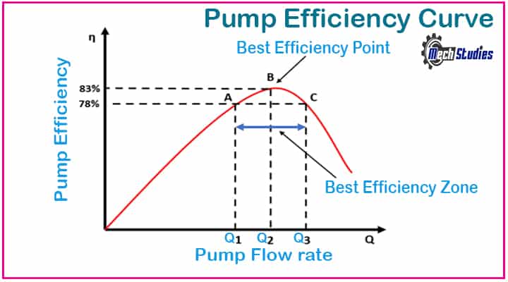
• It is economical to run the pump in the Best Efficiency Zone, the pump operates smoothly in this zone and thus it’s also known as the sweet spot of the pump.
• If the mechanical input of the pump is equal to the pump output in horsepower then the efficiency will be 100 percent. But no pump is 100 efficient, mechanical input is always greater than the output. Efficiency loss occurs due to energy losses caused by friction, leakages due to pressure differentials, etc.
• Pump efficiency is greatest when the largest possible impeller is used, efficiency decreases when smaller impellers are installed as water slips from the gaps between the impeller and pump casing.

Efficiency is given by the following equation –

η_p =P_H/P₂ = ρ . g. Q. H / P₂ x 3600

Where,

• η_p = Pump efficiency
• P_H = Power output of pump
• P₂ = Input power from motor
• ρ = Density of liquid in kg/m³
• g = Acceleration of gravity in m/s²
• Q = Flow in m³/h
• H = Head in m

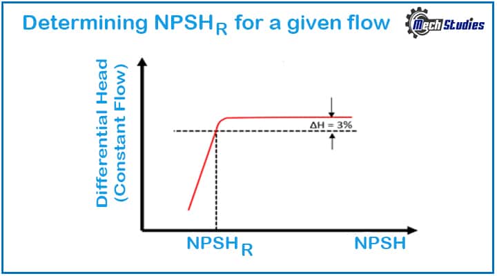
NPSH Curve

• The third curve we will be studying is the Net Positive Suction Head (NPSH) required curve. It provides information about the suction characteristics of the pump at varied flow levels.
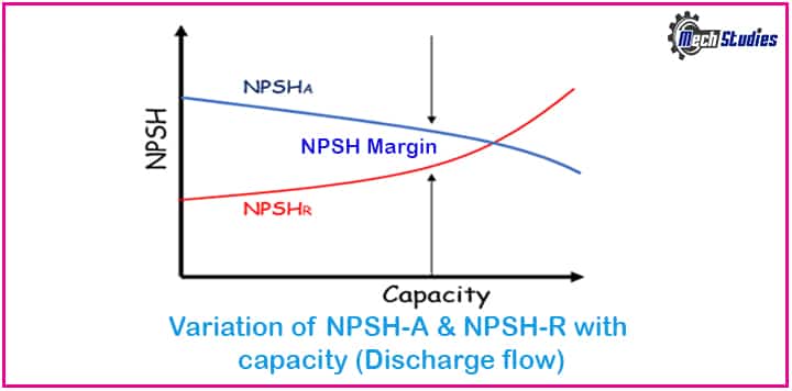
• NPSH is directly proportional to flow, it becomes higher as flow increases and lower when the flow decreases. This means that more pressure head is required at the suction side of the pump for higher flows and vice versa.
• NPSH is independent of the fluid density and is measured in absolute fluid column height.
• The NPSH-R is calculated using water at 20 degrees Celsius. The NPSH-R value is the percentage reduction of 3% in discharged pressure caused by onset cavitation. In a multi-stage pump, only the first set is considered for a 3% pressure drop.

What is NPSH-A?

• NPSH – Available is calculated from the suction side of the pump. It is important that the suction side pressure is less than the vapor pressure of the fluid.
• NPSH-A must exceed NPSH-R for the pump’s working condition to ensure that the cavitation is avoided. A safety margin of 0.5m to 1m is kept to avoid cavitation and for factors such as –
  • Operating environment of the pump
  • Weather changes (Temperature and atmospheric pressure)
  • Increase in friction losses occurring inside the pump
• Safe NPSH margin kept for seamless pump operation. In case of seal-less pumps, minor cavitation can also cause an imbalance in the pump and may cause bearing failures. Thus margins are kept higher

NPSH_available = Ha + ho – hv

Where,

• Ha = suction head at the impeller
• ho = Atmospheric pressure
• hv = Vapor pressure

Ha = h + v²/2g

Where,

• h = Pressure at impeller entrance
• v = Velocity of water at impeller entrance

What is a safe NPSH margin?

• It is described as the safety factor in which the NPSH-A must exceed NPSH-R to avoid cavitation. It can be given by –
  • The ratio of NPSH-A to NPSH-R or
  • Difference between the NPSH-A and NPSH-R. In general conditions, NPSH-A is 0.5m greater than NPSH-R.
• NPSH-A and NPSH-R are not constants, they are the functions of the flow and temperature. When the capacity of the pump changes reassessment of the NPSH margin is required.
  • NPSH-A reduces at high flows due to an increase in frictional losses and head requirements.
  • NPSH-R increases with the flow rate.

How to Generate Pump Curves?

Pump curves are generated by taking measurements of pressure, NPSH, power, efficiency and others, by operating the pump at different flow conditions. The results taken are then plotted against the flow rate to generate the pump characteristics curve.

This method is used when the pump is in working condition, but when the pump is in design phase this method is not suitable. During the design phase various analysis software are used to get the pump you need.

What are Affinity Laws?

The affinity laws are associated with the rotational speed or rpm of the centrifugal pump, if the speed or impeller size changes, the resulted performance change can be given by –

• Flow change is directly proportional to speed: Double the speed – double the flow.
• Pressure changes by the square of difference: Double the speed – pressure increase by four
• Power changes by the cube of difference: Double the speed – Power increase by eight

These laws are applicable for operating points at same efficiency. Impeller diameter variations above 10% are hard to predict due to changes in the relationship between impeller and the pump casing.

High Rated Course

Intro to Fluid Mechanics for Engineering Students Part 1

Intro to Fluid Mechanics for Engineering Students Part 2

Intro to Fluid Mechanics for Engineering Students Part 3

Advanced Fluid Mechanics

Conclusion

Hence, we have got a basic idea about the pump curve. The combination of three curves is called the composite pump curve, together they provide us with the critical information needed to determine if a selected pump is suitable for the hydraulic application.

Understanding the data obtained from the curve is very crucial to guarantee that the pump selected is best suited for hydraulics applications required.

Any comments, please feel free to contact us!